Trigger-based trial selection
Contents
Introduction
This tutorial describes how to define epochs-of-interest (trials) from your recorded MEG-data, and how to apply the different preprocessing steps.
Subsequently, you will find information how to compute an event related potential (ERP)/ event related field (ERF) and how to handle the three channels that record the signal at each sensor location. It explains how to visualize the axial magnetometer and planar gradiometer signals.
Background to preprocessing
In FieldTrip the preprocessing of data refers to the reading of the data, segmenting the data around interesting events such as triggers, temporal filtering and optionally rereferencing. The ft_preprocessing function takes care of all these steps, i.e., it reads the data and applies the preprocessing options.
There are largely two alternative approaches for preprocessing, which especially differ in the amount of memory required. The first approach is to read all data from the file into memory, apply filters, and subsequently cut the data into interesting segments. The second approach is to first identify the interesting segments, read those segments from the data file and apply the filters to those segments only. The remainder of this tutorial explains the second approach, as that is the most appropriate for large data sets such as the MEG data used in this tutorial. The approach for reading and filtering continuous data and segmenting afterwards is explained in another tutorial.
Preprocessing involves several steps including identifying individual trials from the dataset, filtering and artifact rejections. This tutorial covers how to identify trials using the trigger signal. Defining data segments of interest can be done
- according to a specified trigger channel
- according to your own criteria if you write your own trial function
This tutorial will show how you can use the standard FieldTrip functionality for segmenting the data. The concept of the trial function will be introduced and explained in more detail in a follow-up tutorial.
Background to averaging
When analyzing EEG or MEG signals, the aim is to investigate the modulation of the measured brain signals with respect to a certain event. However, due to intrinsic and extrinsic noise in the signals - which in single trials is often higher than the signal evoked by the brain - it is typically required to average data from several trials to increase the signal-to-noise ratio(SNR). One approach is to repeat a given event in your experiment and average the corresponding EEG/MEG signals. The assumption is that the noise is independent of the events and thus reduced when averaging, while the effect of interest is time-locked to the event. The approach results in ERPs and ERFs for respectively EEG and MEG. Timelock analysis can be used to calculate ERPs/ ERFs.
Dataset: MEG median nerve stimulation
The MEG data sets used in this tutorial are two recordings on the same subject during electrical stimulation of the Median Nerve (MN) of the left hand. The reason for the two recordings is that the first recording has a relatively large electrical stimulation artifact, which makes it less suitable for follow-up analysis. The second recording is much cleaner regarding the stimulus artifact, but does not have an experimental manipulation that is of much interest. Hence we will use both.
The first experiment is an oddball task. A regular train of standard stimuli was presented with an occasional oddball. The oddball consisted of a missing stimulus, i.e. there is no stimulus presented at the expected time. The subject was instructed to count the number missing stimuli. In this experiment the oddball manipulation serves two purposes. First it ensures that the subject maintains a constant level attention to the stimulation; we know that the amplitude of the cortical responses depends on the level of attention. Second, the presence of oddballs allows us to study the brain activity related to the expectation of the stimuli.
In the second experiment only normal stimuli were presented in a regular sequence with an inter-stimulus-interval (ISI) that was randomized between 1.9 and 2.1 seconds. The subject did not have an explicit task.
In both cases the MEG signals were recorded with the NatMEG 306 sensor Neuromag Triux system. The Neuromag MEG system has 306 channels located at 102 unique locations in the dewar. Of these, 102 channels are axial magnetometer sensors that measure the magnetic field in the radial direction, i.e. orthogonal to the scalp. The other 2*102 channels are planar gradiometers, which measure the magnetic field gradient tangential to the scalp. The planar gradient MEG data has the advantage that the amplitude typically is the largest directly above a source.
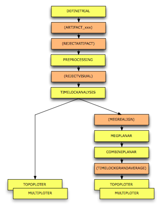
Procedure
The following steps are taken in this tutorial:
- Define segments of data of interest (the trial definition) using ft_definetrial.
- Read the data into MATLAB using ft_preprocessing
- Compute the average over trials using the function ft_preprocessing
- Visualize the results. You can plot the ERF/ ERP of one channel with ft_singleplotER or several channels with ft_multiplotER, or by creating a topographic plot for a specified time- interval with ft_topoplotER.
- Combine the planar gradients for the horizontal and vertical channels.
- Selectively average data in two conditions and compare the ERFs.
Let us start with a clean MATLAB workspace. Since we have two datasets to work with, we will call these dataset "1" and "2". Note that you might have to use the "cd" command to change to the data directory, alternatively you have to specify the full path to the data.
clear all % variables
close all % figures

filename1 = 'somsen_run2_raw_tsss.fif';
filename2 = 'somstim_raw.fif';
Examine the trigger sequence
For an unknown dataset it is often helpful to explore the content of the dataset. Let us start with dataset 2, which is the simplest one.
filename = filename2;
FieldTrip has the high-level functions ft_definetrial and ft_preprocessing for segmenting and reading the data. However, to look at the details of the file, you can use the low-level functions ft_read_header and ft_read_event.
hdr = ft_read_header(filename);
	Read a total of 8 projection items:
		generated with autossp-1.0.1 (1 x 306) idle
		generated with autossp-1.0.1 (1 x 306) idle
		generated with autossp-1.0.1 (1 x 306) idle
		generated with autossp-1.0.1 (1 x 306) idle
		generated with autossp-1.0.1 (1 x 306) idle
		generated with autossp-1.0.1 (1 x 306) idle
		generated with autossp-1.0.1 (1 x 306) idle
		generated with autossp-1.0.1 (1 x 306) idle
	306 MEG channel locations transformed
Opening raw data file somstim_raw.fif...
	Read a total of 8 projection items:
		generated with autossp-1.0.1 (1 x 306) idle
		generated with autossp-1.0.1 (1 x 306) idle
		generated with autossp-1.0.1 (1 x 306) idle
...
You see a lot of (debugging) information on screen. Let us look at the relevant information:
disp(hdr);
          label: {324x1 cell}
         nChans: 324
             Fs: 1000
           grad: [1x1 struct]
       nSamples: 826000
    nSamplesPre: 0
        nTrials: 1
           orig: [1x1 struct]
       chantype: {324x1 cell}
       chanunit: {324x1 cell}
There are 324 channels, sampled at 1000 Hz. The channel labels are
disp(hdr.label');
  Columns 1 through 6

    'BIO001'    'BIO002'    'BIO003'    'BIO004'    'IASX+'    'IASX-'

  Columns 7 through 13

    'IASY+'    'IASY-'    'IASZ+'    'IASZ-'    'IAS_DX'    'IAS_DY'    'IAS_X'

  Columns 14 through 19

    'IAS_Y'    'IAS_Z'    'MEG0111'    'MEG0112'    'MEG0113'    'MEG0121'

  Columns 20 through 25

    'MEG0122'    'MEG0123'    'MEG0131'    'MEG0132'    'MEG0133'    'MEG0141'
...
which get interesting from channel 16 onwards. If you pay close attention, you can see that the naming scheme groups the channels into triplets. More information is available in hdr.chantype and hdr.chanunit.
disp(hdr.chantype')
  Columns 1 through 6

    'unknown'    'unknown'    'unknown'    'unknown'    'unknown'    'unknown'

  Columns 7 through 12

    'unknown'    'unknown'    'unknown'    'unknown'    'unknown'    'unknown'

  Columns 13 through 17

    'unknown'    'unknown'    'unknown'    'megmag'    'megplanar'

  Columns 18 through 22

    'megplanar'    'megmag'    'megplanar'    'megplanar'    'megmag'
...
disp(hdr.chanunit')
  Columns 1 through 11

    'V'    'V'    'V'    'V'    'V'    'V'    'V'    'V'    'V'    'V'    'V'

  Columns 12 through 21

    'V'    'V'    'V'    'V'    'T'    'T/m'    'T/m'    'T'    'T/m'    'T/m'

  Columns 22 through 30

    'T'    'T/m'    'T/m'    'T'    'T/m'    'T/m'    'T'    'T/m'    'T/m'

  Columns 31 through 39

    'T'    'T/m'    'T/m'    'T'    'T/m'    'T/m'    'T'    'T/m'    'T/m'
...
Knowing what is contained in the file according to the header is a good starting point. Now we have to figure out what trigger codes were used in the experiment and whether the experiment can be reconstructed given the data file.
event = ft_read_event(filename);
	Read a total of 8 projection items:
		generated with autossp-1.0.1 (1 x 306) idle
		generated with autossp-1.0.1 (1 x 306) idle
		generated with autossp-1.0.1 (1 x 306) idle
		generated with autossp-1.0.1 (1 x 306) idle
		generated with autossp-1.0.1 (1 x 306) idle
		generated with autossp-1.0.1 (1 x 306) idle
		generated with autossp-1.0.1 (1 x 306) idle
		generated with autossp-1.0.1 (1 x 306) idle
	306 MEG channel locations transformed
Opening raw data file somstim_raw.fif...
	Read a total of 8 projection items:
		generated with autossp-1.0.1 (1 x 306) idle
		generated with autossp-1.0.1 (1 x 306) idle
		generated with autossp-1.0.1 (1 x 306) idle
...
Again there is a lot of (debugging) information on screen, which you can ignore. Each event in this dataset represents a single trigger, which is characterized by a trigger value (the code) and the sample (time at which it happened).
event(1)
ans =

        type: 'STI101'
      sample: 12284
       value: 1
      offset: []
    duration: []
event(2)
ans =

        type: 'STI101'
      sample: 14343
       value: 1
      offset: []
    duration: []
We can reorganize them and visualize the sequence of triggers in a graph:
sample = [event.sample]; % make a vector of all sample numbers
value  = [event.value];  % make a vector of all trigger values
plot(sample/hdr.Fs, value, '.')
xlabel('time (s)')
ylabel('trigger value')
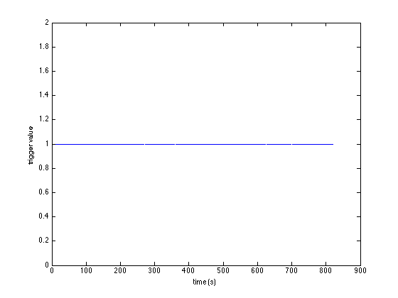
It looks like a line, but actually is a large number of points.
INSTRUCTION: Use the MATLAB "zoom in" function to look at the points detail. You see that there is only a single type of stimulus with trigger code 1. We can look at it in more detail with
plot(diff(sample)/hdr.Fs, '.')
xlabel('number')
ylabel('ISI (s)')
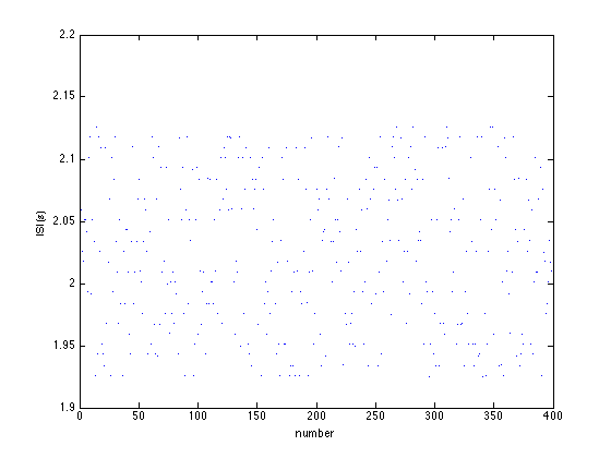
Now you see that the inter-stimulus interval varies slightly.
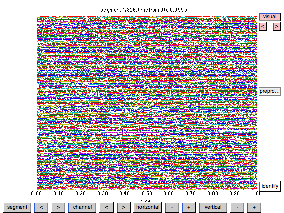
Rather than looking at details of the data, a possibility is also to just look at the MEG timeseries themselves. This can be done with the data still on disk, i.e. prior to preprocessing, using ft_databrowser. The databrowser allows you to scroll through data, and optionally to mark sections as artifactual.
cfg = [];
cfg.dataset = filename;
cfg.channel = 'MEGGRAD';
cfg.preproc.demean = 'yes';
cfg.viewmode = 'vertical';
ft_databrowser(cfg);
	Read a total of 8 projection items:
		generated with autossp-1.0.1 (1 x 306) idle
		generated with autossp-1.0.1 (1 x 306) idle
		generated with autossp-1.0.1 (1 x 306) idle
		generated with autossp-1.0.1 (1 x 306) idle
		generated with autossp-1.0.1 (1 x 306) idle
		generated with autossp-1.0.1 (1 x 306) idle
		generated with autossp-1.0.1 (1 x 306) idle
		generated with autossp-1.0.1 (1 x 306) idle
	306 MEG channel locations transformed
Opening raw data file somstim_raw.fif...
	Read a total of 8 projection items:
		generated with autossp-1.0.1 (1 x 306) idle
		generated with autossp-1.0.1 (1 x 306) idle
		generated with autossp-1.0.1 (1 x 306) idle
...
Let us continue processing this data. First we define which segments of data are of interest:
cfg = [];
cfg.dataset   = filename;
cfg.trialfun  = 'ft_trialfun_general';
cfg.trialdef.eventtype  = 'STI101';
cfg.trialdef.eventvalue = 1;
cfg.trialdef.prestim    = 0.050; % in seconds
cfg.trialdef.poststim   = 0.250; % in seconds
cfg = ft_definetrial(cfg);
evaluating trialfunction 'ft_trialfun_general'
	Read a total of 8 projection items:
		generated with autossp-1.0.1 (1 x 306) idle
		generated with autossp-1.0.1 (1 x 306) idle
		generated with autossp-1.0.1 (1 x 306) idle
		generated with autossp-1.0.1 (1 x 306) idle
		generated with autossp-1.0.1 (1 x 306) idle
		generated with autossp-1.0.1 (1 x 306) idle
		generated with autossp-1.0.1 (1 x 306) idle
		generated with autossp-1.0.1 (1 x 306) idle
	306 MEG channel locations transformed
Opening raw data file somstim_raw.fif...
	Read a total of 8 projection items:
		generated with autossp-1.0.1 (1 x 306) idle
		generated with autossp-1.0.1 (1 x 306) idle
...
This results in an updated cfg structure. The important field is cfg.trl, which contains in the 1st column the begin sample of each segment of interest, in the 2nd column the end sample and in the 3rd column it contains the number of samples with which the time axis should be shifted relative to the start of the segment. In this case we have 50 samples in the data segment prior to the trigger (and the stimulus) being present.
disp(cfg.trl)
       12234       12533         -50           1
       14293       14592         -50           1
       16319       16618         -50           1
       18337       18636         -50           1
       20388       20687         -50           1
       22439       22738         -50           1
       24481       24780         -50           1
       26474       26773         -50           1
       28575       28874         -50           1
       30693       30992         -50           1
       32685       32984         -50           1
       34736       35035         -50           1
       36770       37069         -50           1
       38696       38995         -50           1
       40822       41121         -50           1
...
Subsequently we proceed actually reading the data into memory. We could use the low-level FieldTrip function ft_read_data for this, but it is more convenient to use the high-level ft_preprocessing function, which offers a large collection of preprocessing options for the data.
Here we specify that we want to remove the mean value that is estimated in the baseline, i.e. the time window prior to stimulation.
cfg.baselinewindow = [-inf 0];
cfg.demean         = 'yes';
data = ft_preprocessing(cfg);
	Read a total of 8 projection items:
		generated with autossp-1.0.1 (1 x 306) idle
		generated with autossp-1.0.1 (1 x 306) idle
		generated with autossp-1.0.1 (1 x 306) idle
		generated with autossp-1.0.1 (1 x 306) idle
		generated with autossp-1.0.1 (1 x 306) idle
		generated with autossp-1.0.1 (1 x 306) idle
		generated with autossp-1.0.1 (1 x 306) idle
		generated with autossp-1.0.1 (1 x 306) idle
	306 MEG channel locations transformed
Opening raw data file somstim_raw.fif...
	Read a total of 8 projection items:
		generated with autossp-1.0.1 (1 x 306) idle
		generated with autossp-1.0.1 (1 x 306) idle
		generated with autossp-1.0.1 (1 x 306) idle
...
INSTRUCTION: Have a look at the data structure and try to understand the various fields:
disp(data)
           hdr: [1x1 struct]
         label: {324x1 cell}
          time: {1x400 cell}
         trial: {1x400 cell}
       fsample: 1000
    sampleinfo: [400x2 double]
     trialinfo: [400x1 double]
          grad: [1x1 struct]
           cfg: [1x1 struct]
The most important fields are 'data.trial' containing the individual trials and 'data.time' containing the time vector for each trial. Details on the data structure are available in the help of http://fieldtrip.fcdonders.nl/reference/ft_datatype_rawft_datatype_raw.
To visualize the single trial data (trial 1) on one channel (channel 130) do the following using plain MATLAB code:
figure
plot(data.time{1}, data.trial{1}(130,:));
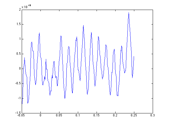
The figure of channel 130 (which is 'MEG1111') shows quite some oscillatory noise.
QUESTION: Compare channel MEG1111 with MEG1112 and MEG1113. What is the source of the noise on channel MEG1111?
This would be a good moment to store the intermediate result to disk.
save somsens2_data.mat data
Timelockanalysis
The function ft_timelockanalysis makes averages of all the trials in a data structure. It requires preprocessed data (see
load somsens2_data.mat
All trials in the data structure will now be averaged with the onset of the stimulus time aligned to the zero-time point (the onset of the MN stimulus). This is done with the function ft_timelockanalysis. The input to this procedure is the data structure generated by ft_preprocessing. No special settings are necessary here, thus specify an empty configuration.
cfg = [];
avg = ft_timelockanalysis(cfg, data);
the input is raw data with 324 channels and 400 trials
averaging trials
averaging trial 400 of 400

the call to "ft_timelockanalysis" took 3 seconds and required the additional allocation of an estimated 2 MB
The output is the "avg" structure with the following fields:
disp(avg);
       avg: [324x300 double]
       var: [324x300 double]
      time: [1x300 double]
       dof: [324x300 double]
     label: {324x1 cell}
    dimord: 'chan_time'
      grad: [1x1 struct]
       cfg: [1x1 struct]
It is possible to make subselections of channels for averaging (or in any other analysis), e.g.
cfg = [];
cfg.channel = 'MEGMAG';
avg_mag = ft_timelockanalysis(cfg, data);

cfg = [];
cfg.channel = 'MEGGRAD';
avg_planar = ft_timelockanalysis(cfg, data);
the input is raw data with 324 channels and 400 trials
averaging trials
averaging trial 400 of 400

the call to "ft_timelockanalysis" took 1 seconds and required the additional allocation of an estimated 1 MB
the input is raw data with 324 channels and 400 trials
averaging trials
averaging trial 400 of 400

the call to "ft_timelockanalysis" took 1 seconds and required the additional allocation of an estimated 0 MB
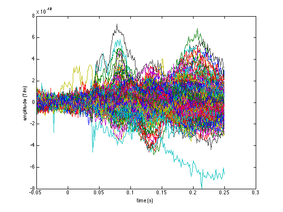
The averaged data can be visualized using standard MATLAB functions like this
figure
plot(avg_mag.time, avg_mag.avg);
xlabel('time (s)');
ylabel('amplitude (T)');

figure
plot(avg_planar.time, avg_planar.avg);
xlabel('time (s)');
ylabel('amplitude (T/m)');
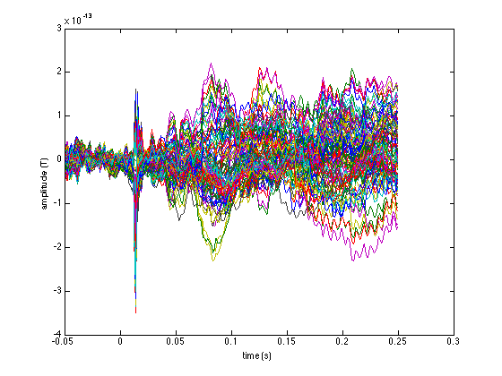
Note the different units along the vertical axes. These explain why the following figure is not very interpretable:
figure
plot(avg.time, avg.avg);
xlabel('time (s)');
ylabel('amplitude (a.u.)');
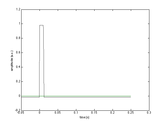
In this figure you mainly see one large "block", which is the (averaged) trigger channel with value 1. Other channels are numerically much smaller and don't show individually, unless you zoom in.
The interpretation of the data is much easier if you plot all data on the approximate location of the channels. FieldTrip allows a very flexible layout of channels in the plots, to accomodate MEG, EEG, ECoG, LFP and other types of data, all coming from very different acquisition systems. The layout of channels is explained in this tutorial. For the Neuromag system, we provide the following template layouts:
- neuromag306all.lay (all channels, split in triplets)
- neuromag306mag.lay (only magnetometer channels, at the actual location)
- neuromag306planar.lay (only planar channels, split in pairs)
- neuromag306cmb.lay (combined planar channels, at the actual location)
cfg = [];
cfg.layout = 'neuromag306mag.lay';
figure;
ft_multiplotER(cfg, avg_mag);

cfg.layout = 'neuromag306planar.lay';
figure;
ft_multiplotER(cfg, avg_planar);
selection avg along dimension 1
selection dof along dimension 1
selection var along dimension 1
reading layout from file neuromag306mag.lay
the call to "ft_prepare_layout" took 0 seconds and required the additional allocation of an estimated 0 MB
the call to "ft_multiplotER" took 2 seconds and required the additional allocation of an estimated 2 MB
selection avg along dimension 1
selection dof along dimension 1
selection var along dimension 1
reading layout from file neuromag306planar.lay
the call to "ft_prepare_layout" took 0 seconds and required the additional allocation of an estimated 0 MB
the call to "ft_multiplotER" took 3 seconds and required the additional allocation of an estimated 4 MB
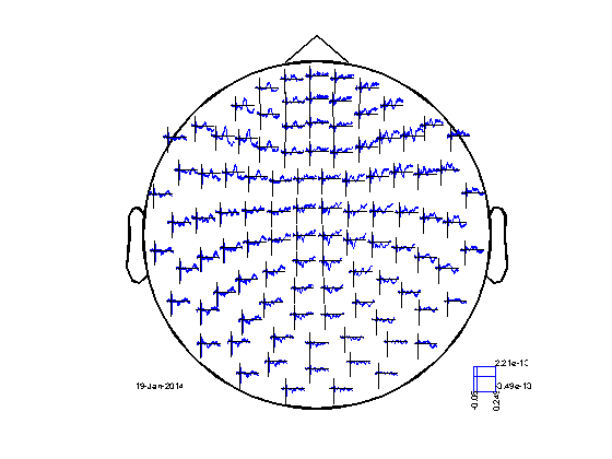

INSTRUCTION: Using your mouse, you can make selections in the "avg_mag" figure and click in the selection. This will give you a new figure, zooming in on the selected aspects of the data (channels or time).
NOTE: you can also make the same selections in the "avg_planar" figure. However, you will see that the topographical display looks weird. Try to explain the unusual structure in the topography.
Rather than looking at the horizontal and vertical planar gradient separately, we can combine the planar channels into one "magnitude" estimate using ft_combineplanar. For ERFs this is done using Pythagoras' rule, i.e. c = sqrt(a^2+b^2) where a and b are the planar gradients in the two directions and c the magnitude. In this representation you loose the information of the direction of the gradient.
cfg = [];
avg_cmb = ft_combineplanar(cfg, avg_planar);

cfg = [];
cfg.layout = 'neuromag306cmb.lay';
figure;
ft_multiplotER(cfg, avg_cmb);
the input is timelock data with 204 channels and 300 timebins
the input is timelock data with 204 channels and 300 timebins
Warning: the trial definition in the configuration is inconsistent with the
actual data
Warning: reconstructing sampleinfo by assuming that the trials are consecutive
segments of a continuous recording
the input is raw data with 102 channels and 1 trials
the call to "ft_combineplanar" took 1 seconds and required the additional allocation of an estimated 1 MB
selection avg along dimension 1
reading layout from file neuromag306cmb.lay
the call to "ft_prepare_layout" took 0 seconds and required the additional allocation of an estimated 0 MB
the call to "ft_multiplotER" took 1 seconds and required the additional allocation of an estimated 3 MB
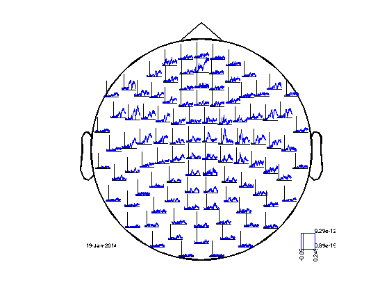
INSTRUCTION: Use the interactive feature of the figure to make a selection and try to plot the topography for the earliest SEF response.
Again, this would be a good time to save your intermediate results:
save somsens2_avg_mag.mat     avg_mag
save somsens2_avg_planar.mat  avg_planar
save somsens2_avg_cmb.mat     avg_cmb
Examine a more complex trigger sequence
Let us continue with dataset 1, which consists of standard stimuli and missing stimuli as oddballs.
filename = filename1;
Again we can look at the content of the file using the low-level reading functions:
hdr = ft_read_header(filename);

disp(hdr)
	306 MEG channel locations transformed
Opening raw data file somsen_run2_raw_tsss.fif...
	Range : 743000 ... 998999  =    743.000 ...   998.999 secs
Ready.
          label: {322x1 cell}
         nChans: 322
             Fs: 1000
           grad: [1x1 struct]
       nSamples: 256000
    nSamplesPre: 0
        nTrials: 1
           orig: [1x1 struct]
       chantype: {322x1 cell}
       chanunit: {322x1 cell}
event = ft_read_event(filename);

disp(event)
	306 MEG channel locations transformed
Opening raw data file somsen_run2_raw_tsss.fif...
	Range : 743000 ... 998999  =    743.000 ...   998.999 secs
Ready.
Reading 743000 ... 998999  =    743.000 ...   998.999 secs... [done]
600x1 struct array with fields:
    type
    sample
    value
    offset
    duration
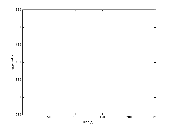
There are 600 events in this dataset. We can reorganize their representation in MATLAB and visualize the sequence of triggers in a graph:
sample = [event.sample]; % make a vector of all sample numbers
value  = [event.value];  % make a vector of all trigger values
plot(sample/hdr.Fs, value, '.')
xlabel('time (s)')
ylabel('trigger value')

You can see that there are two trigger values: 256 and 512, and that 256 is more frequent:
sum(value==256)
sum(value==512)
ans =

   500


ans =

   100
Compare ERFs over conditions
It is possible to process the standards and the deviants separately like this
cfg = [];
cfg.dataset   = filename;
cfg.trialfun  = 'ft_trialfun_general';
cfg.trialdef.eventtype  = 'STI101';
cfg.trialdef.eventvalue = 256;
cfg.trialdef.prestim    = 0.050; % in seconds
cfg.trialdef.poststim   = 0.250; % in seconds
cfg = ft_definetrial(cfg);

cfg.baselinewindow = [-inf 0];
cfg.demean         = 'yes';
standard = ft_preprocessing(cfg);
evaluating trialfunction 'ft_trialfun_general'
	306 MEG channel locations transformed
Opening raw data file somsen_run2_raw_tsss.fif...
	Range : 743000 ... 998999  =    743.000 ...   998.999 secs
Ready.
reading the events from 'somsen_run2_raw_tsss.fif'
	306 MEG channel locations transformed
Opening raw data file somsen_run2_raw_tsss.fif...
	Range : 743000 ... 998999  =    743.000 ...   998.999 secs
Ready.
Reading 743000 ... 998999  =    743.000 ...   998.999 secs... [done]
found 600 events
created 500 trials
the call to "ft_definetrial" took 5 seconds and required the additional allocation of an estimated 0 MB
	306 MEG channel locations transformed
...
cfg = [];
cfg.dataset   = filename;
cfg.trialfun  = 'ft_trialfun_general';
cfg.trialdef.eventtype  = 'STI101';
cfg.trialdef.eventvalue = 512;
cfg.trialdef.prestim    = 0.050; % in seconds
cfg.trialdef.poststim   = 0.250; % in seconds
cfg = ft_definetrial(cfg);

cfg.baselinewindow = [-inf 0];
cfg.demean         = 'yes';
deviant = ft_preprocessing(cfg);
evaluating trialfunction 'ft_trialfun_general'
	306 MEG channel locations transformed
Opening raw data file somsen_run2_raw_tsss.fif...
	Range : 743000 ... 998999  =    743.000 ...   998.999 secs
Ready.
reading the events from 'somsen_run2_raw_tsss.fif'
	306 MEG channel locations transformed
Opening raw data file somsen_run2_raw_tsss.fif...
	Range : 743000 ... 998999  =    743.000 ...   998.999 secs
Ready.
Reading 743000 ... 998999  =    743.000 ...   998.999 secs... [done]
found 600 events
created 100 trials
the call to "ft_definetrial" took 5 seconds and required the additional allocation of an estimated 0 MB
	306 MEG channel locations transformed
...

disp(standard)
disp(deviant)
           hdr: [1x1 struct]
         label: {322x1 cell}
          time: {1x500 cell}
         trial: {1x500 cell}
       fsample: 1000
    sampleinfo: [500x2 double]
     trialinfo: [500x1 double]
          grad: [1x1 struct]
           cfg: [1x1 struct]

           hdr: [1x1 struct]
         label: {322x1 cell}
          time: {1x100 cell}
         trial: {1x100 cell}
       fsample: 1000
...
However, if you want to do a fair comparison between the two experimental conditions (e.g. to study anticipation), it is better to ensure that you treat them exactly the same. Especially relevant is the potentially subjective selection of trials to exclude due to artifacts: since you have fewer deviants than standards, you might be tempted to use a slightly more leniant threshold for artifact detection in the deviants. This can introduce a potential bias between the two conditions which invalidates later comparisons.
Instead, you can do
cfg = [];
cfg.dataset   = filename;
cfg.trialfun  = 'ft_trialfun_general';
cfg.trialdef.eventtype  = 'STI101';
cfg.trialdef.eventvalue = [256 512]; % select both triggers
cfg.trialdef.prestim    = 0.050;
cfg.trialdef.poststim   = 0.250;
cfg = ft_definetrial(cfg);

cfg.baselinewindow = [-inf 0];
cfg.demean         = 'yes';
data = ft_preprocessing(cfg);
evaluating trialfunction 'ft_trialfun_general'
	306 MEG channel locations transformed
Opening raw data file somsen_run2_raw_tsss.fif...
	Range : 743000 ... 998999  =    743.000 ...   998.999 secs
Ready.
reading the events from 'somsen_run2_raw_tsss.fif'
	306 MEG channel locations transformed
Opening raw data file somsen_run2_raw_tsss.fif...
	Range : 743000 ... 998999  =    743.000 ...   998.999 secs
Ready.
Reading 743000 ... 998999  =    743.000 ...   998.999 secs... [done]
found 600 events
created 600 trials
the call to "ft_definetrial" took 5 seconds and required the additional allocation of an estimated 0 MB
	306 MEG channel locations transformed
...
to get the data from both condictions in one raw data structure.
disp(data)
           hdr: [1x1 struct]
         label: {322x1 cell}
          time: {1x600 cell}
         trial: {1x600 cell}
       fsample: 1000
    sampleinfo: [600x2 double]
     trialinfo: [600x1 double]
          grad: [1x1 struct]
           cfg: [1x1 struct]
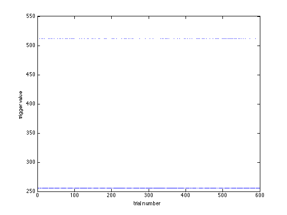
The field data.trialinfo now becomes relevant, as it contains the trigger code of each of the two conditions:
figure
plot(data.trialinfo, '.');
xlabel('trial number')
ylabel('trigger value')
Although an elaborate artifact handling is outside the scope of this tutorial, a quick visual inspection and rejection of bad trials can be done using ft_rejectvisual:
cfg = [];
cfg.method = 'summary';
cfg.channel = 'MEGMAG';
cfg.layout = 'neuromag306mag.lay';
dataclean = ft_rejectvisual(cfg, data);
the input is raw data with 322 channels and 600 trials
showing a summary of the data for all channels and trials
computing metric [---------------------------------------------------------]
588 trials marked as GOOD, 12 trials marked as BAD
102 channels marked as GOOD, 220 channels marked as BAD
the following trials were removed: 39, 60, 61, 68, 121, 130, 161, 201, 324, 326, 338, 410
the following channels were removed: EOG001, EOG002, ECG003, IASX+, IASX-, IASY+, IASY-, IASZ+, IASZ-, IAS_DX, IAS_DY, IAS_X, IAS_Y, IAS_Z, MEG0112, MEG0113, MEG0122, MEG0123, MEG0132, MEG0133, MEG0142, MEG0143, MEG0212, MEG0213, MEG0222, MEG0223, MEG0232, MEG0233, MEG0242, MEG0243, MEG0312, MEG0313, MEG0322, MEG0323, MEG0332, MEG0333, MEG0342, MEG0343, MEG0412, MEG0413, MEG0422, MEG0423, MEG0432, MEG0433, MEG0442, MEG0443, MEG0512, MEG0513, MEG0522, MEG0523, MEG0532, MEG0533, MEG0542, MEG0543, MEG0612, MEG0613, MEG0622, MEG0623, MEG0632, MEG0633, MEG0642, MEG0643, MEG0712, MEG0713, MEG0722, MEG0723, MEG0732, MEG0733, MEG0742, MEG0743, MEG0812, MEG0813, MEG0822, MEG0823, MEG0912, MEG0913, MEG0922, MEG0923, MEG0932, MEG0933, MEG0942, MEG0943, MEG1012, MEG1013, MEG1022, MEG1023, MEG1032, MEG1033, MEG1042, MEG1043, MEG1112, MEG1113, MEG1122, MEG1123, MEG1132, MEG1133, MEG1142, MEG1143, MEG1212, MEG1213, MEG1222, MEG1223, MEG1232, MEG1233, MEG1242, MEG1243, MEG1312, MEG1313, MEG1322, MEG1323, MEG1332, MEG1333, MEG1342, MEG1343, MEG1412, MEG1413, MEG1422, MEG1423, MEG1432, MEG1433, MEG1442, MEG1443, MEG1512, MEG1513, MEG1522, MEG1523, MEG1532, MEG1533, MEG1542, MEG1543, MEG1612, MEG1613, MEG1622, MEG1623, MEG1632, MEG1633, MEG1642, MEG1643, MEG1712, MEG1713, MEG1722, MEG1723, MEG1732, MEG1733, MEG1742, MEG1743, MEG1812, MEG1813, MEG1822, MEG1823, MEG1832, MEG1833, MEG1842, MEG1843, MEG1912, MEG1913, MEG1922, MEG1923, MEG1932, MEG1933, MEG1942, MEG1943, MEG2012, MEG2013, MEG2022, MEG2023, MEG2032, MEG2033, MEG2042, MEG2043, MEG2112, MEG2113, MEG2122, MEG2123, MEG2132, MEG2133, MEG2142, MEG2143, MEG2212, MEG2213, MEG2222, MEG2223, MEG2232, MEG2233, MEG2242, MEG2243, MEG2312, MEG2313, MEG2322, MEG2323, MEG2332, MEG2333, MEG2342, MEG2343, MEG2412, MEG2413, MEG2422, MEG2423, MEG2432, MEG2433, MEG2442, MEG2443, MEG2512, MEG2513, MEG2522, MEG2523, MEG2532, MEG2533, MEG2542, MEG2543, MEG2612, MEG2613, MEG2622, MEG2623, MEG2632, MEG2633, MEG2642, MEG2643, STI101, SYS201
the call to "ft_rejectvisual" took 16 seconds and required the additional allocation of an estimated 49 MB
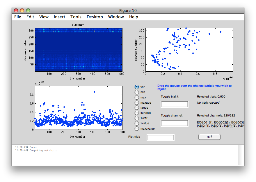
INSTRUCTION: Please select all trials with a variance that exceeds 5e10^-25 in the lower left panel of the figure. If you select from the menu View->Figure Toolbar, you can use the zoom button to identify individual trials or channels with a large amount of variance, such as trial 410, and make a topographic plot of such an individial trial tro try and understand the nature of the artifacts.
Following artifact rejection, you can compute ERFs of the two conditions separately:
cfg = [];
cfg.trials = dataclean.trialinfo==256;
avg_std = ft_timelockanalysis(cfg, dataclean);
the input is raw data with 102 channels and 588 trials
selecting 491 trials
averaging trials
averaging trial 491 of 491

the call to "ft_timelockanalysis" took 1 seconds and required the additional allocation of an estimated 0 MB
cfg = [];
cfg.trials = dataclean.trialinfo==512;
avg_dev = ft_timelockanalysis(cfg, dataclean);
the input is raw data with 102 channels and 588 trials
selecting 97 trials
averaging trials
averaging trial 97 of 97

the call to "ft_timelockanalysis" took 0 seconds and required the additional allocation of an estimated 1 MB
and plot them together:
cfg = [];
cfg.channel = 'MEGMAG';
cfg.layout = 'neuromag306mag.lay';
figure
ft_multiplotER(cfg, avg_std, avg_dev);
selection avg along dimension 1
selection dof along dimension 1
selection var along dimension 1
selection avg along dimension 1
selection dof along dimension 1
selection var along dimension 1
reading layout from file neuromag306mag.lay
the call to "ft_prepare_layout" took 0 seconds and required the additional allocation of an estimated 0 MB
the call to "ft_multiplotER" took 1 seconds and required the additional allocation of an estimated 2 MB
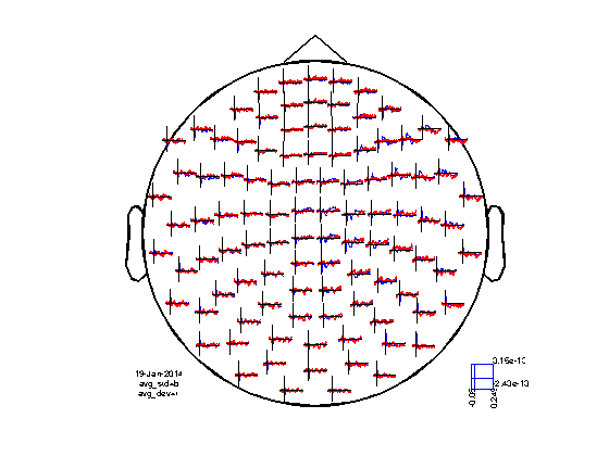
Note that the effect of the expectation of the stimulus is small, but seems to be visible in the ERFs.
save somsens2_dataclean.mat dataclean
save somsens2_avg_std.mat   avg_std
save somsens2_avg_dev.mat   avg_dev
Summary and suggested further reading
This tutorial covered trial selection, preprocessing and event-related averaging of MEG data. Furthermore, it showed the difference between magnetometer and planar channels and how to plot the results.
One important aspect of MEG preprocessing which was not covered here in detail is removing artifacts and cleaning the data. On the FieldTrip website you can find information on how to deal with artifacts. Furthermore, the ft_databrowser is a helpful function to explore quality of the data.
After calculating the ERFs for each condition and comparing them by eye, a relevant next step is to test if there are statistically significant differences in the ERF amplitudes. If you are interested in this, you can continue with the event-related statistics tutorial.
If you are interested in a different analysis of your data that shows event related changes in the oscillatory components of the signal, you can continue with the time-frequency analysis tutorial.