Cluster-based permutation tests on event related fields

Contents

Introduction

The objective of this tutorial is to give an introduction to the statistical analysis of event-related EEG and MEG data (denoted as MEEG data in the following) by means of cluster-based permutation tests. The tutorial starts with a long background section that sketches the background of permutation tests. Subsequently it is shown how to use FieldTrip to perform cluster-based permutation tests on single-channel time-frequency decomposed data in a between-trials (within-subject) design.

In this tutorial we will continue working on the visual stimulus dataset we used before in the timefrequency tutorials. Below we will repeat code to select the trials and preprocess the data. We assume that the preprocessing and frequency analysis steps of the analysis are already clear for the reader.

This tutorial is not covering statistical test on event-related fields. If you are interested in that, you can read the Cluster-based permutation tests on ERF tutorial. If you are interested in a more gentle introduction as to how parametric statistical tests can be used with FieldTrip, you can read the Parametric and non-parametric statistics on event-related fields tutorial.

Background

The multiple comparisons problem In the statistical analysis of MEEG-data we have to deal with the multiple comparisons problem (MCP). This problem originates from the fact that MEEG-data are multidimensional. MEEG-data have a spatiotemporal structure: the signal is sampled at multiple channels and multiple time points (as determined by the sampling frequency). The MCP arises from the fact that the effect of interest (i.e., a difference between experimental conditions) is evaluated at an extremely large number of (channel,time)-pairs. This number is usually in the order of several thousands. Now, the MCP involves that, due to the large number of statistical comparisons (one per (channel,time)-pair), it is not possible to control the so called family-wise error rate (FWER) by means of the standard statistical procedures that operate at the level of single (channel,time)-pairs. The FWER is the probability under the hypothesis of no effect of falsely concluding that there is a difference between the experimental conditions at one or more (channel,time)-pairs. A solution of the MCP requires a procedure that controls the FWER at some critical alpha-level (typically, 0.05 or 0.01). The FWER is also called the false alarm rate.

In this tutorial, we describe nonparametric statistical testing of MEEG-data. Contrary to the familiar parametric statistical framework, it is straightforward to solve the MCP in the nonparametric framework. Fieldtrip contains a set of statistical functions that provide a solution for the MCP. These are the functions ft_timelockstatistics and ft_freqstatistics which compute significance probabilities using a non-parametric permutation tests. Besides nonparametric statistical tests, ft_timelockstatistics and ft_freqstatistics can also perform parametric statistical tests (see the Parametric and non-parametric statistics on ERFs tutorial). However, in this tutorial the focus will be on non-parametric testing.

Structure in experiment and data

Different types of data

MEEG-data have a spatiotemporal structure: the signal is sampled at multiple channels and multiple time points. Thus, MEEG-data are two-dimensional: channels (the spatial dimension) X time-points (the temporal dimension). In the following, these (channel,time)-pairs will be called samples. In some studies, these two-dimensional data are reduced to one-dimensional data by averaging over either a selected set of channels or a selected set of time-points.

In many studies, there is an interest in the modulation of oscillatory brain activity. Oscillatory brain activity is measured by power estimates obtained from Fourier or wavelet analyses of single-trial spatiotemporal data. Very often, power estimates are calculated for multiple data segments obtained by sliding a short time window over the complete data segment. In this way, spatio-spectral-temporal data are obtained from the raw spatiotemporal data. The spectral dimension consists of the different frequency bins for which the power is calculated. In the following, these (channel,frequency,time)-triplets will be called samples. In some studies, these three-dimensional data are reduced to one- or two-dimensional data by averaging over a selected set of channels, a selected set of time points, and/or a selected set of frequencies.

Structure in an experiment

The data are typically collected in different experimental conditions and the experimenter wants to know if there is a significant difference between the data observed in these conditions. To answer this question, statistical tests are used. To understand these statistical tests one has to know how the structure in the experiment affects the structure in the data. Two concepts are crucial for describing the structure in an experiment:

The concept of a unit of observation (UO). The concept of a between- or a within-UO design. In MEEG experiments, there are two types of UO: subjects and trials (i.e., epochs of time within a subject). Concerning the concept of a between- or a within-UO design, there are two schemes according to which the UOs can be assigned to the experimental conditions: (1) every UO is assigned to only one of a number of experimental conditions (between UO-design; independent samples), or (2) every UO is assigned to multiple experimental conditions in a particular order (within UO-design; dependent samples). Therefore, in a between-UO design, there is only one experimental condition per UO, and in a within-UO design there are multiple experimental conditions per UO. These two experimental designs require different test statistics.

The two UO-types (subjects and trials) and the two experimental designs (between- and within-UO) can be combined and this results in four different types of experiments.

Computation of the test statistic and its significance probability

The statistical testing in FieldTrip is performed by the functions ft_timelockstatistics, ft_freqstatistics and ft_sourcestatistics. From a statistical point of view, the calculations performed by these functions are very similar. They only differ in the data handling and with respect to the data structures on which they operate: ft_timelockstatistics operates on data structures produced by ft_timelockanalysis and ft_timelockgrandaverage, and ft_freqstatistics operates on data structures produced by ft_freqanalysis, ft_freqgrandaverage, and ft_freqdescriptives.

To correct for multiple comparisons, one has to specify the field cfg.correctm. This field can have the values 'no', 'max', 'cluster', 'bonferoni', 'holms', or 'fdr'. In this tutorial, we only use cfg.correctm = 'cluster', which solves the MCP by calculating a so-called cluster-based test statistic and its significance probability.

The calculation of the significance probability

If the MCP is solved by choosing for a cluster-based test statistic (i.e., with cfg.correctm = 'cluster'), the significance probability can only be calculated by means of the so-called Monte Carlo method. This is because the reference distribution for a permutation test can be approximated (to any degree of accuracy) by means of the Monte Carlo method. In the configuration, the Monte Carlo method is chosen as follows: cfg.method = 'montecarlo'.

The Monte Carlo significance probability is calculated differently for a within- and between-UO design. We now show how the Monte Carlo significance probability is calculated for in a between-trials experiment (a between-UO design with trials as UO):

If the p-value is smaller than the critical alpha-level (typically 0.05) then we conclude that the data in the two experimental conditions are significantly different. This p-value can also be calculated for the second largest cluster-level statistic, the third largest, etc. It is common practice to say that a cluster is significant if its p-value is less than the critical alpha-level. This practice suggests that it is possible to do spatio-spectral-temporal localization by means of the cluster-based permutation test. However, from a biophysical perspective, this suggestion is not justified. Consult Maris and Oostenveld, Journal of Neuroscience Methods, 2007 for an elaboration on this topic.

Procedure

In this tutorial we will consider a between-trials experiment, in which we analyze the data of a single subject. The statistical analysis for this experiment we perform both on axial and planar ERFs. The steps we perform are as follows:

The dataset

We will continue to work on the dataset of teh visual change-detection experiment. Magneto-encephalography (MEG) data was collected using the 306-channel Neuromag Triux MEG system at NatMEG. The subject was instructed to fixate on the screen and press a left- or right-hand button upon a speed change of an inward moving stimulus Each trial started with the presentation of a cue pointing either rightward or leftward, indicating the response hand. Subsequently a fixation cross appeared. After a baseline interval of 1s, an inward moving circular sine-wave grating was presented. After an unpredictable delay, the grating changed speed, after which the subjects had to press a button with the cued hand. In a small fraction of the trials there was no speed change and subjects should not respond.

The dataset allows for a number of different questions, e.g.

These questions require different analysis strategies on different sections of the data. In this analysis we will focuss on question 1, i.e. the effect of cueuing in absence of overt motor activity.

Defining data segments of interest

The first step is to read the data using the function ft_preprocessing, which requires the specification of the trials by ft_definetrial. Due to the complex nature of the trigger sequence, we use a custom trial function

edit trialfun_visual_cue

This trialfun_visual_cue function is defined such that it takes the cfg structure as input, and produces a 'trl' matrix as output. Furthermore, it returns the event structure.

function [trl, event] = trialfun_visual_cue(cfg)

The code of this function makes use of the cfg.dataset field and of cfg.trialdef.pre = time before the first trigger cfg.trialdef.post = time after the last trigger

clear all
close all

filename = 'workshop_visual_sss.fif';

cfg = [];
cfg.dataset   = filename;
cfg.trialfun  = 'trialfun_visual_cue';
cfg.trialdef.pre  = 0.500; % prior to the cue
cfg.trialdef.post = 0.000; % following the stimulus onset
cfg = ft_definetrial(cfg);

cfg.channel = 'MEGGRAD';
cfg.demean = 'yes';
cfg.baselinewindow = [-inf 0];
data = ft_preprocessing(cfg);

evaluating trialfunction 'trialfun_visual_cue'
Warning: adding /Users/robert/matlab/fieldtrip/external/mne toolbox to your
Matlab path 
==============================================================================

Copyright (c) 2011, Matti Hamalainen and Alexandre Gramfort
All rights reserved.

Redistribution and use in source and binary forms, with or without
modification, are permitted provided that the following conditions are met:
    * Redistributions of source code must retain the above copyright
      notice, this list of conditions and the following disclaimer.
    * Redistributions in binary form must reproduce the above copyright
      notice, this list of conditions and the following disclaimer in the
      documentation and/or other materials provided with the distribution.
...

Using ft_rejectvisual we can perform a quick scan of the overall data quality and exclude noisy trials:

cfg             = [];
cfg.method      = 'summary';
cfg.keepchannel = 'yes';
dataclean = ft_rejectvisual(cfg, data);

the input is raw data with 204 channels and 125 trials
showing a summary of the data for all channels and trials
computing metric [--------------------------------------------------------\]
122 trials marked as GOOD, 3 trials marked as BAD
204 channels marked as GOOD, 0 channels marked as BAD
the following trials were removed: 6, 10, 74
the call to "ft_rejectvisual" took 49 seconds and required the additional allocation of an estimated 10 MB

Time-frequency analysis

To speed up the subsequent computations and reduce memory requirements, we will downsample the data from 1000 to 250 Hz. This is not recommended for normal analysis, where you would better wait a bit longer. However, for the sake of the hands-on tutorial we want to the analyses to run fast.

cfg = [];
cfg.resamplefs  = 250;
cfg.demean      = 'no';
cfg.detrend     = 'no';
resampled = ft_resampledata(cfg, dataclean);

the input is raw data with 204 channels and 122 trials
resampling data
resampling data in trial 122 from 122

original sampling rate = 1000 Hz
new sampling rate = 250 Hz
the call to "ft_resampledata" took 3 seconds and required the additional allocation of an estimated 84 MB

For the time-frequency analysis, we will use a wavelet decomposition. Since we want to compute a statistical contrast between the left- and right-hand cue, we need to keep the spectral estimates for each trial rather than compute the average over all trials.

cfg = [];
cfg.method  = 'wavelet';
cfg.keeptrials = 'yes'; % keep the spectral estimates for each trial
cfg.pad     = 2;
cfg.toi     = -0.500:0.0500:0.750;
cfg.foi     = 2:2:70;
cfg.gwidth  = 3;
cfg.width   = 5;
TFRwavelet  = ft_freqanalysis(cfg, resampled);

the input is raw data with 204 channels and 122 trials
Warning: the trial definition in the configuration is inconsistent with the
actual data 
Warning: reconstructing sampleinfo by assuming that the trials are consecutive
segments of a continuous recording 
processing trials
Warning: output time-bins are different from input time-bins 
trial 122, frequency 35 (70.00 Hz)

the call to "ft_freqanalysis" took 33 seconds and required the additional allocation of an estimated 160 MB

This computation takes a few minutes.

It is possible to perform statistical tests on all channels, using spatial clustering. However, for reaons of efficiency we will now pick a single channel that shows a motor-preparation effect and only consider that channel. It still requires us to consider multiple comparisons, as there are many timepoints and frequencies. Also clustering is still possible along the time- and frequency-dimensions.

cfg = [];
cfg.layout        = 'neuromag306planar.lay';
cfg.baselinetype  = 'relchange';
cfg.baseline      = [-inf 0];
cfg.renderer      = 'painters'; % the default is OpenGL, which is faster, but it gives visual artifacts on some computers
cfg.colorbar      = 'yes';
figure
ft_multiplotTFR(cfg, TFRwavelet);

the input is freq data with 204 channels, 35 frequencybins and 26 timebins
the call to "ft_freqdescriptives" took 0 seconds and required the additional allocation of an estimated 1 MB
reading layout from file neuromag306planar.lay
the call to "ft_prepare_layout" took 0 seconds and required the additional allocation of an estimated 1 MB
the input is freq data with 204 channels, 35 frequencybins and 26 timebins
the call to "ft_freqbaseline" took 0 seconds and required the additional allocation of an estimated 0 MB
Warning: (one of the) axis is/are not evenly spaced, but plots are made as if
axis are linear 
the call to "ft_multiplotTFR" took 5 seconds and required the additional allocation of an estimated 17 MB

Note that we have NOT combined the two planar channels, so you should not use the interactive mode to make the power topography. We can use the MATLAB zoom function to zoom in on the channels overlying motor areas and subsequently select one of the channels.

One channel that shows a cue-related response in the beta band is channel MEG1243 over the right motor areas.

cfg = [];
cfg.channel       = {'MEG1243'};
cfg.baselinetype  = 'relchange';
cfg.baseline      = [-inf 0];
cfg.renderer      = 'painters'; % the default is OpenGL, which is faster, but it gives visual artifacts on some computers
cfg.colorbar      = 'yes';
figure
ft_singleplotTFR(cfg, TFRwavelet);

the input is freq data with 204 channels, 35 frequencybins and 26 timebins
the call to "ft_freqdescriptives" took 0 seconds and required the additional allocation of an estimated 2 MB
the input is freq data with 204 channels, 35 frequencybins and 26 timebins
the call to "ft_freqbaseline" took 0 seconds and required the additional allocation of an estimated 2 MB
the call to "ft_singleplotTFR" took 1 seconds and required the additional allocation of an estimated 0 MB

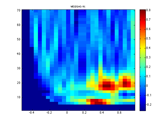
Sofar we have been looking at the average of both left- and right-conditions. With ft_freqanalysis we did compute single-trial TFRs, but the plotting functions average it on the fly. Having identified a channel, being blind for the contrast of interest, we can now ask the question whether this channel shows differential activity depending on cue direction.

The field TFRwavelet.trialinfo contains the code for the left and right hand trials, so we can start by making selective averages for the two.

cfg = [];
cfg.channel       = {'MEG1243'};
cfg.baselinetype  = 'relchange';
cfg.baseline      = [-inf 0];
cfg.renderer      = 'painters'; % the default is OpenGL, which is faster, but it gives visual artifacts on some computers
cfg.colorbar      = 'yes';
cfg.zlim          = [-1 1];     % use the same scaling for both figures

cfg.trials        = TFRwavelet.trialinfo(:,1)==1;
figure
ft_singleplotTFR(cfg, TFRwavelet);
title('cue towards left');

cfg.trials        = TFRwavelet.trialinfo(:,1)==2;
figure
ft_singleplotTFR(cfg, TFRwavelet);
title('cue towards right');

the input is freq data with 204 channels, 35 frequencybins and 26 timebins
selection powspctrm along dimension 1
the call to "ft_freqdescriptives" took 0 seconds and required the additional allocation of an estimated 95 MB
the input is freq data with 204 channels, 35 frequencybins and 26 timebins
the call to "ft_freqbaseline" took 0 seconds and required the additional allocation of an estimated 0 MB
the call to "ft_singleplotTFR" took 1 seconds and required the additional allocation of an estimated 95 MB
the input is freq data with 204 channels, 35 frequencybins and 26 timebins
selection powspctrm along dimension 1
the call to "ft_freqdescriptives" took 0 seconds and required the additional allocation of an estimated 0 MB
the input is freq data with 204 channels, 35 frequencybins and 26 timebins
the call to "ft_freqbaseline" took 0 seconds and required the additional allocation of an estimated 1 MB
the call to "ft_singleplotTFR" took 1 seconds and required the additional allocation of an estimated 2 MB

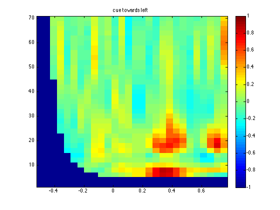
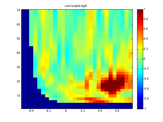
The two averages show a potential effect, which means that I am not making a nonsense script up at 23.00 in the evening ;-) Normally you should not look at the differences in the data to identify a region of interest, as it will bias your results towards finding false positives. Let us continue with the formal comparisons of the two conditions as if nothing happened.

Statistical testing

Cluster-level permutation tests for time-frequency representations are performed by the function ft_freqstatistics. This function takes as its arguments a configuration (cfg) and one or more data structures. These data structures must be produced by ft_freqanalysis or ft_freqgrandaverage, which all operate on preprocessed data.

The configuration settings

Some fields of the configuration (cfg), such as channel and latency, are not specific for ft_freqstatistics; their role is similar in other FieldTrip functions.

cfg = [];
cfg.method            = 'montecarlo';           % use the Monte Carlo Method to calculate the significance probability
cfg.statistic         = 'indepsamplesT';        % use the independent samples T-statistic as a measure to evaluate the effect at the sample level
cfg.correctm          = 'cluster';
cfg.clusteralpha      = 0.05;                   % alpha level of the sample-specific test statistic that will be used for thresholding
cfg.clustertail       = 0;
cfg.clusterstatistic  = 'maxsum';               % test statistic that will be evaluated under the permutation distribution.
cfg.tail              = 0;                      % -1, 1 or 0 (default = 0); one-sided or two-sided test
cfg.correcttail       = 'prob';                 % the two-sided test implies that we do non-parametric two tests
cfg.alpha             = 0.05;                   % alpha level of the permutation test
cfg.numrandomization  = 1000;                   % number of draws from the permutation distribution
cfg.design            = TFRwavelet.trialinfo(:,1)'; % design matrix, note the transpose
cfg.ivar              = 1;                      % the index of the independent variable in the design matrix
cfg.channel           = {'MEG1243'};
cfg.neighbours        = [];                     % there are no spatial neighbours, only in time and frequency

We now describe the most relevant options one-by-one.

The help in the ft_statistics_montecarlo function explains these in detail.

Having explained the relevance of the configuration options, let us proceed with the actual computation.

stat = ft_freqstatistics(cfg, TFRwavelet);

computing statistic over the frequency range [2.000 70.000]
computing statistic over the time range [-0.500 0.752]
the call to "ft_appendfreq" took 0 seconds and required the additional allocation of an estimated 171 MB
selection powspctrm along dimension 2
selection powspctrm along dimension 3
selection powspctrm along dimension 4
using "ft_statistics_montecarlo" for the statistical testing
using "ft_statfun_indepsamplesT" for the single-sample statistics
constructing randomized design
total number of measurements     = 122
total number of variables        = 1
number of independent variables  = 1
number of unit variables         = 0
number of within-cell variables  = 0
number of control variables      = 0
...

The format of the output

disp(stat)

                   prob: [1x35x26 double]
            posclusters: [1x6 struct]
    posclusterslabelmat: [1x35x26 double]
        posdistribution: [1x1000 double]
            negclusters: [1x5 struct]
    negclusterslabelmat: [1x35x26 double]
        negdistribution: [1x1000 double]
                cirange: [1x35x26 double]
                   mask: [1x35x26 logical]
                   stat: [1x35x26 double]
                    ref: [1x35x26 double]
                 dimord: 'chan_freq_time'
                  label: {'MEG1243'}
                   freq: [1x35 double]
                   time: [1x26 double]
...

You see that the structure is not dissimilar to the TFR-structure, except there are now multiple fields with the dimord 'chan_freq_time' (where you should note that we have one channel due to the a-priori selection).

Since the structure is in general the same, we can use the same plotting function for the results of the statistics as for the TFR itself:

cfg = [];
cfg.channel       = {'MEG1243'};
cfg.baseline      = [-inf 0];
cfg.renderer      = 'painters';
cfg.colorbar      = 'yes';
cfg.parameter     = 'stat'; % display the statistical value, i.e. the t-score
figure
ft_singleplotTFR(cfg, stat);
title('t-score (not corrected)')

the input is freq data with 1 channels, 35 frequencybins and 26 timebins
the call to "ft_freqbaseline" took 0 seconds and required the additional allocation of an estimated 0 MB
the call to "ft_singleplotTFR" took 1 seconds and required the additional allocation of an estimated 1 MB

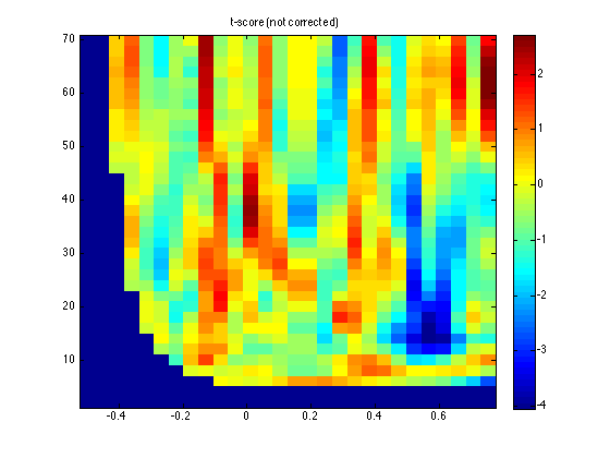
This shows the massive-univariate statistical value that was computed, i.e. 'indepsamplesT'.

The relevant answer to the question: is there a significant difference is found in the mask, i.e. the binary representation of the statistical test:

disp(any(stat.mask(:)))

     1

This reveals that there is indeed a significant effect somewhere in the 35x26 time-frequency points that we considered.

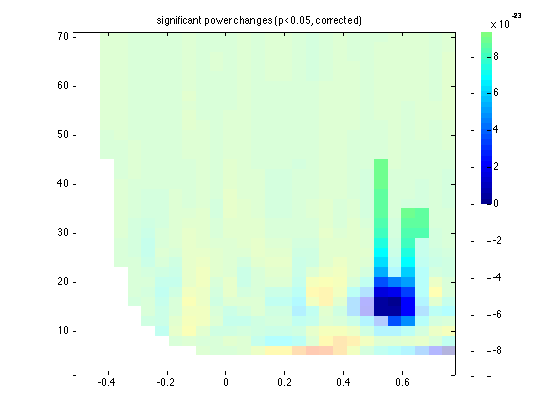
We can (manually) compute the raw effect, i.e. the difference in means and use the mask field to plot the masked raw effect.

chansel  = find(strcmp(TFRwavelet.label, 'MEG1243')); % find the channel index
leftsel  = TFRwavelet.trialinfo(:,1)==1;              % select the left trials
rightsel = TFRwavelet.trialinfo(:,1)==2;              % select the right trials
powspctrm_left  = mean(TFRwavelet.powspctrm(leftsel,chansel,:,:), 1);
powspctrm_right = mean(TFRwavelet.powspctrm(rightsel,chansel,:,:), 1);

effect = powspctrm_left - powspctrm_right;
siz    = size(effect);
effect = reshape(effect, siz(2:end)); % we need to "squeeze" out one of the dimensions, i.e. make it 3-D rather than 4-D

We can add the raw effect to the stat structure, now that it has the same dimensions as stat.stat, stat.prob and stat.mask.

Note that the raw effect is expressed in units of the original data, not as a ratio.

stat.effect = effect;

cfg = [];
cfg.channel       = {'MEG1243'};
cfg.baseline      = [-inf 0];
cfg.renderer      = 'openGL';     % painters does not support opacity, openGL does
cfg.colorbar      = 'yes';
cfg.parameter     = 'effect';     % display the power
cfg.maskparameter = 'mask';       % use significance to mask the power
cfg.maskalpha     = 0.3;          % make non-significant regions 30% visible
cfg.zlim          = 'maxabs';
figure
ft_singleplotTFR(cfg, stat);
title('significant power changes (p<0.05, corrected)')

the input is freq data with 1 channels, 35 frequencybins and 26 timebins
the call to "ft_freqbaseline" took 0 seconds and required the additional allocation of an estimated 0 MB
the call to "ft_singleplotTFR" took 0 seconds and required the additional allocation of an estimated 0 MB

INSTRUCTION: repeat the statistical test, but now as a parametric test. This is realized by specifying cfg.method='analytic' in ft_freqstatistics. See also ft_statistics_analytic.

cfg = [];
cfg.method            = 'analytic';             % calculate the analytic significance probability
cfg.statistic         = 'indepsamplesT';        % use the independent samples T-statistic as a measure to evaluate the effect at the sample level
cfg.tail              = 0;
cfg.alpha             = 0.05;                   % alpha level of the (single) parametric test
cfg.design            = TFRwavelet.trialinfo';  % design matrix, note the transpose
cfg.ivar              = 1;                      % the index of the independent variable in the design matrix
cfg.channel           = {'MEG1243'};

% using no correction for multiple comparisons
cfg.correctm          = 'no';
statpar_no = ft_freqstatistics(cfg, TFRwavelet);

% using Bonferroni correction for multiple comparisons
cfg.correctm          = 'bonferroni';
statpar_bf = ft_freqstatistics(cfg, TFRwavelet);

% using False Discovery Rate correction for multiple comparisons
cfg.correctm          = 'fdr';
statpar_fdr = ft_freqstatistics(cfg, TFRwavelet);

computing statistic over the frequency range [2.000 70.000]
computing statistic over the time range [-0.500 0.752]
the call to "ft_appendfreq" took 0 seconds and required the additional allocation of an estimated 171 MB
selection powspctrm along dimension 2
selection powspctrm along dimension 3
selection powspctrm along dimension 4
using "ft_statistics_analytic" for the statistical testing
using "ft_statfun_indepsamplesT" for the single-sample statistics
Warning: Not all replications are used for the computation of the statistic. 
not performing a correction for multiple comparisons
the call to "ft_freqstatistics" took 1 seconds and required the additional allocation of an estimated 171 MB
computing statistic over the frequency range [2.000 70.000]
computing statistic over the time range [-0.500 0.752]
the call to "ft_appendfreq" took 0 seconds and required the additional allocation of an estimated 172 MB
selection powspctrm along dimension 2
...

Again we can add the raw effect to the stat structure and use the mask field to visualize the time-frequency points that were found to be significance (ignoring multiple comparisons).

statpar_no.effect = effect;

cfg = [];
cfg.channel       = {'MEG1243'};
cfg.baseline      = [-inf 0];
cfg.renderer      = 'openGL';     % painters does not support opacity, openGL does
cfg.colorbar      = 'yes';
cfg.parameter     = 'prob';       % display the power
cfg.maskparameter = 'mask';       % use significance to mask the power
cfg.maskalpha     = 0.3;          % make non-significant regions 30% visible
cfg.zlim          = 'maxabs';
figure
ft_singleplotTFR(cfg, statpar_no);

title('significant power changes (p<0.05, not corrected)')

the input is freq data with 1 channels, 35 frequencybins and 26 timebins
the call to "ft_freqbaseline" took 0 seconds and required the additional allocation of an estimated 0 MB
the call to "ft_singleplotTFR" took 0 seconds and required the additional allocation of an estimated 0 MB

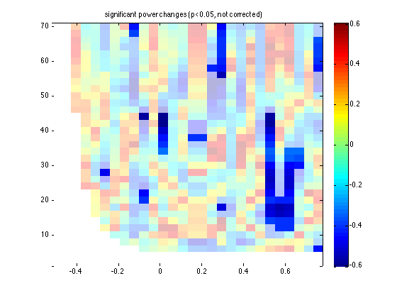
You see that the same late region is found as significant, but also some scattered time-frequency points elsewhere.

An interesting question is what would happen if the data were truely random. We can simulate this by randomizing the design, i.e. randomizing the assignment of the original data over the left and right condition.

cfg = [];
cfg.method            = 'analytic';             % calculate the analytic significance probability
cfg.statistic         = 'indepsamplesT';        % use the independent samples T-statistic as a measure to evaluate the effect at the sample level
cfg.tail              = 0;
cfg.alpha             = 0.05;                   % alpha level of the (single) parametric test
cfg.design            = TFRwavelet.trialinfo(:,1)'; % design matrix, note the transpose

shuffle = randperm(length(cfg.design))

cfg.design            = cfg.design(:,shuffle);  % shuffle the left and right trials

cfg.ivar              = 1;                      % the index of the independent variable in the design matrix
cfg.channel           = {'MEG1243'};

shuffle =

  Columns 1 through 13

    86   113    29   120    80    65    51    32    87    45    47    98   102

  Columns 14 through 26

    24    18    46    63    27   118    74    17    95   110   114    56    82

  Columns 27 through 39

   105    34    64    30    72    36     9     8    19    67    20    16   101

...

use no correction for multiple comparisons

cfg.correctm          = 'no';
statpar_falsealarm = ft_freqstatistics(cfg, TFRwavelet);

computing statistic over the frequency range [2.000 70.000]
computing statistic over the time range [-0.500 0.752]
the call to "ft_appendfreq" took 0 seconds and required the additional allocation of an estimated 170 MB
selection powspctrm along dimension 2
selection powspctrm along dimension 3
selection powspctrm along dimension 4
using "ft_statistics_analytic" for the statistical testing
using "ft_statfun_indepsamplesT" for the single-sample statistics
Warning: Not all replications are used for the computation of the statistic. 
not performing a correction for multiple comparisons
the call to "ft_freqstatistics" took 1 seconds and required the additional allocation of an estimated 170 MB

Again we can add the raw effect to the stat structure and use the mask field to visualize the time-frequency points that were found to be significance (ignoring multiple comparisons). You can see that there it a considerable number of false alarms.

statpar_falsealarm.effect = effect;

INSTRUCTION: You can try the same test for the control of the false alarm rate for the clustering, Bonferroni and the FDR methods for multiple comparison corrections. If you were to repeat the false alarm test 100 times, ideally you would get a significant effect (in the absence of any effect) in no more than 5%, i.e. at or below the alpha level.

INSTRUCTION: In all computations above we used indepsamplesT as the massive univariate statistic. This statistic is implemented in a stand-alone function, just like the trialfuns are. In this case it is "ft_statfun_indepsamplesT.m".

edit ft_statfun_indepsamplesT

There are more example functions provided in fieldtrip/statfun, at which you can have a look. You can also provide your own function, which can make the test more sensitive to the specific effects you expect to be in the data. This "statfun" acts as the black box as discussed in the statistics lecture.

Summary and suggested further readings

In this tutorial, we showed how to do non-parametric statistical test, cluster-based permutation test on TFR's with a between-trials experimental design. It was also shown how to plot the results.

If you are interested in parametric tests in FieldTrip, you can read the Parametric and non-parametric statistics on event-related fields tutorial. If you want to get more details on time-frequency tests, we suggest you follow the Cluster-based permutation tests on time-frequency data tutorial. If you are interested in how to do the same statistics on event-related fields, you can read the Cluster-based permutation tests on event related fields tutorial.

Published with MATLAB® R2012b